Animating diffusion processes in networks

NotebookLM Summary

../assets/audio/notebooklm_network_diffusion.wav

Overview

1. NDlib at a Glance
2. Generating Diffusion Plots Per Timestep
3. FuncAnimation to Animate Plots Over Time
4. NDlib Model and Network Configuration
5. Observing Code Updates in the Widget
6. Voila Webapp

NDlib at a Glance

NDlib is a Python library designed for modeling and simulating diffusion processes over complex networks. It provides a variety of epidemic and information diffusion models, such as SIR, SIS, and Independent Cascade, which can be applied to networks created using libraries like NetworkX. NDlib simplifies the process of configuring, running, and visualizing these models, making it an excellent tool for researchers and educators.

For example, here’s how we define a simple SIR model using NDlib:

import networkx as nx
import ndlib.models.ModelConfig as mc
import ndlib.models.epidemics as ep

# Create a graph
g = nx.erdos_renyi_graph(10, 0.2)

# Define the SIR model
model = ep.SIRModel(g)

# Configure the model parameters
cfg = mc.Configuration()
cfg.add_model_parameter('beta', 0.5)  # Infection rate
cfg.add_model_parameter('gamma', 0.1)  # Recovery rate
cfg.add_model_parameter("fraction_infected", 0.2)  # Initial infected fraction
model.set_initial_status(cfg)

# Run the model for a number of timesteps
iterations = model.iteration_bunch(20)

---

Generating Diffusion Plots Per Timestep

NDlib provides tools to visualize the diffusion process over time. For example, we can use the DiffusionTrend class to plot the number of susceptible, infected, and recovered nodes at each timestep.

from ndlib.viz.mpl.DiffusionTrend import DiffusionTrend

# Generate trends from the model's iterations
trends = model.build_trends(iterations)

# Visualize the trends
viz = DiffusionTrend(model, trends)
viz.plot()

This produces a static plot showing how the diffusion evolves over time.

---

FuncAnimation to Animate Plots Over Time

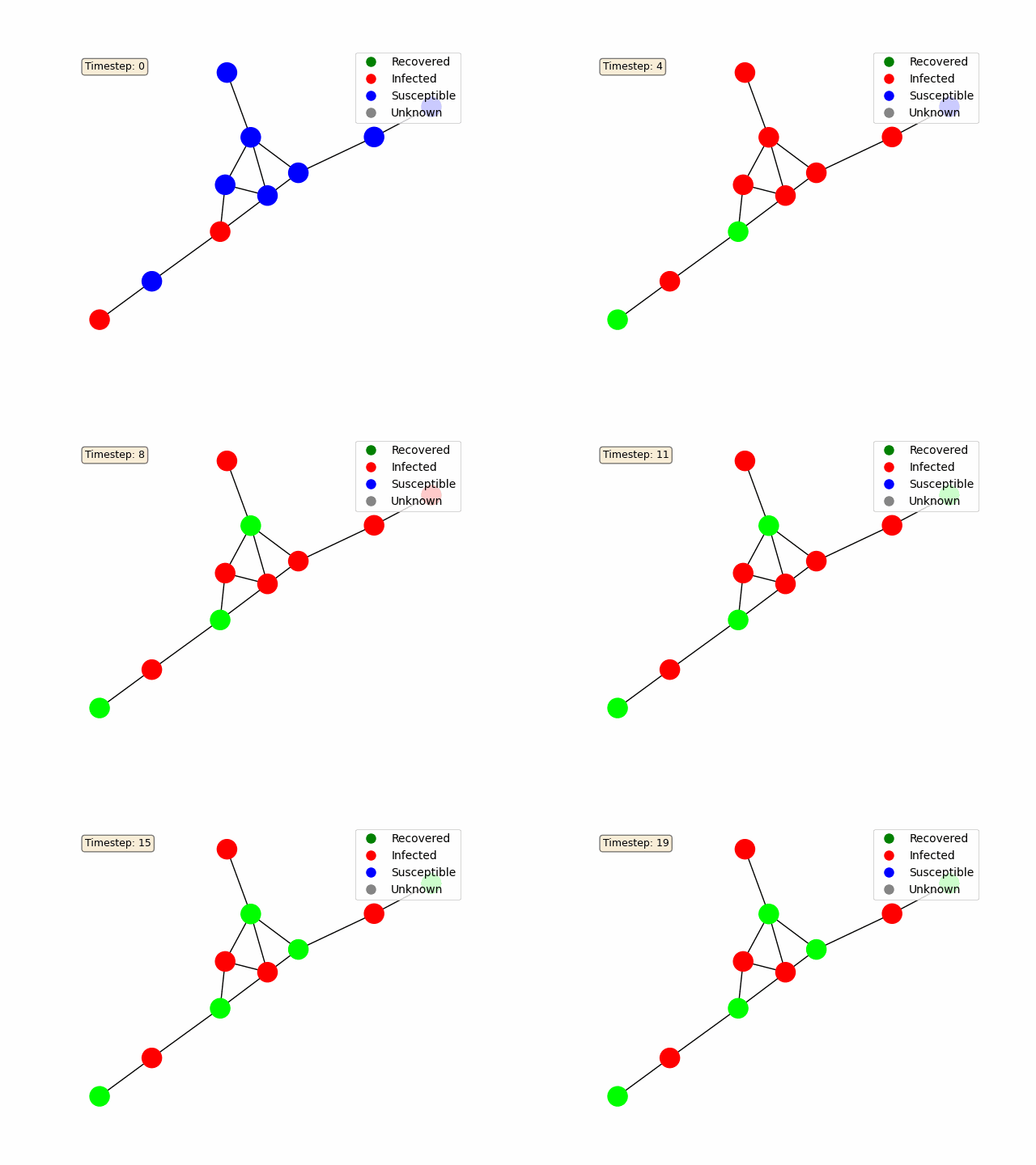
To make the diffusion process more interactive, we use Matplotlib’s FuncAnimation to animate the network’s state over time. Each node is colored based on its status (e.g., blue for susceptible, red for infected, green for recovered).

import matplotlib.pyplot as plt
from matplotlib.animation import FuncAnimation

# Define node colors based on their status
def get_node_colors(status):
    colors = []
    for node in status.keys():
        if status[node] == 0:
            colors.append('blue')  # Susceptible
        elif status[node] == 1:
            colors.append('red')  # Infected
        elif status[node] == 2:
            colors.append('green')  # Recovered
    return colors

# Prepare the animation
fig, ax = plt.subplots()
pos = nx.spring_layout(g)
nodes = nx.draw_networkx_nodes(g, pos, node_color=get_node_colors(iterations[0]['status']), ax=ax)
edges = nx.draw_networkx_edges(g, pos, ax=ax)

def update(frame):
    current_state = iterations[frame]['status']
    nodes.set_facecolor(get_node_colors(current_state))
    return nodes,

animation = FuncAnimation(fig, update, frames=len(iterations), interval=500, blit=True)
plt.show()

For a basic random graph as in the example above, you should get something like this:

NDlib Model and Network Configuration

To make the simulation interactive, we use Jupyter widgets. Users can modify the model’s parameters and the number of timesteps using a text area and a slider.

import ipywidgets as widgets
from IPython.display import display

# Text area for modifying the model code
code_input = widgets.Textarea(
    value="""def get_iterations(g, time_steps):
    model = ep.SIRModel(g)
    cfg = mc.Configuration()
    cfg.add_model_parameter('beta', 0.5)
    cfg.add_model_parameter('gamma', 0.1)
    cfg.add_model_parameter("fraction_infected", 0.2)
    model.set_initial_status(cfg)
    return model.iteration_bunch(time_steps), model
""",
    layout=widgets.Layout(width='100%', height='300px')
)

# Slider for adjusting the number of timesteps
time_steps_slider = widgets.IntSlider(
    value=20,
    min=1,
    max=100,
    step=1,
    description='Time Steps:'
)

# Display the widgets
display(code_input)
display(time_steps_slider)

These widgets enable users to experiment with different network configurations and model parameters without modifying the underlying code.

---

Observing Code Updates in the Widget

The line code_input.observe(run_code, names='value') is used to observe changes in the code_input widget. Whenever the user modifies the code in the text area, the run_code function is triggered. This is necessary because:

1. Dynamic Updates: It allows the application to dynamically re-run the simulation whenever the user changes the code or parameters.
2. Interactivity: Without this observation, the user would need to manually trigger the simulation, reducing the interactivity of the application.
3. Error Handling: The run_code function can handle errors in the user-provided code, ensuring the application remains responsive even if invalid code is entered.

Here’s how the observation is set up:

def run_code(change):
    with output:
        try:
            clear_output(wait=True)
            local_vars = {}
            exec(change['new'], globals(), local_vars)
            get_iterations = local_vars['get_iterations']
            iterations, model = get_iterations(g, time_steps_slider.value)
            # Additional logic for updating plots and animations...
        except Exception as e:
            print("Error executing code:", e)

# Observe changes in the code input
code_input.observe(run_code, names='value')

This ensures that the application reacts immediately to user input, providing a seamless interactive experience.

---

Voila Webapp

Finally, we use Voila to convert the notebook into a standalone web application. Voila renders the notebook as an interactive dashboard, hiding the code cells and displaying only the widgets, plots, and animations. This makes it easy to share the application with others, even if they don’t have Python or Jupyter installed.

To run the web app, simply execute the following command in the terminal:

voila [network_animation.ipynb](https://github.com/PeterCarragher/diffusion_animator/blob/master/network_animation.ipynb)

This will launch a browser window where users can interact with the diffusion simulation, modify parameters, and observe the results in real-time.

---

By combining NDlib, Matplotlib, Jupyter widgets, and Voila, this notebook provides a powerful and interactive tool for visualizing diffusion processes in networks. It serves as both an educational resource and a platform for experimentation. For the full code, checkout this Github repository.